Static models
The examples use the packages, the MCMC settings and the Serie A 2000/2001 data created in Get started:
library(footBayes)
library(dplyr)
library(ggplot2)
library(bayesplot)
library(loo)

n_iter <- 1000
n_chains <- 4
seed <- 2026

data("italy")
italy <- as.data.frame(italy)

italy_2000 <- italy %>%
  filter(Season == "2000") %>%
  arrange(Date) %>%
  select(periods = Season, home_team = home, away_team = visitor,
         home_goals = hgoal, away_goals = vgoal)
This article shows how to fit static goal-based models and how to read their estimates. In a static model, the attack and defence abilities of each team are constant over the whole period covered by the data. The models are fitted to the 306 matches of the 2000/2001 Serie A, first by maximum likelihood and then in a Bayesian framework; two further sections show how to change the prior distributions and the inference algorithm.
| Function / argument | What it does | Output |
|---|---|---|
mle_foot() |
Maximum likelihood estimation | A list with the estimates, their 95% confidence intervals, the log-likelihood, AIC and BIC |
stan_foot() |
Bayesian estimation with Stan | An object of class stanFoot, containing the CmdStanFit object |
print() |
Posterior summaries of a stanFoot object |
A table with one row per parameter |
prior_par (argument of stan_foot()) |
Changes the prior distributions | - |
method (argument of stan_foot()) |
Changes the inference algorithm (MCMC, variational inference, Pathfinder, Laplace) | - |
How static models work
The models are presented in Goal-based models in a nutshell. For the models of the goal counts (double and bivariate Poisson, Dixon-Coles, negative binomial) and for the Skellam model, the scoring rates of the home and the away team in match \(n\) are
\[\log(\lambda_{1n}) = \text{home} + \text{att}_{h_n} + \text{def}_{a_n}, \qquad \log(\lambda_{2n}) = \text{att}_{a_n} + \text{def}_{h_n},\]
where \(h_n\) and \(a_n\) are the home and the away team (the Student-\(t\) model replaces the attack and defence abilities with a single overall ability per team). There is no intercept, and the abilities satisfy a sum-to-zero constraint, so that they are measured with respect to an average team with \(\text{att} = \text{def} = 0\). Hence:
- a positive attack ability means that the team scores more than an average team against the same opponent;
- a negative defence ability means that the team concedes fewer goals than an average team: the defence of the opponent enters the scoring rate with a plus sign, so the lower the better;
- the home effect acts multiplicatively: for two teams with the same abilities, the home scoring rate is \(\exp\{\text{home}\}\) times the away one.
The two estimation routes treat the abilities differently. mle_foot() treats the abilities as fixed parameters with no prior and maximizes the likelihood. stan_foot() treats the abilities as exchangeable, with a common prior whose standard deviations \(\sigma_{\text{att}}, \sigma_{\text{def}}\) are estimated from the data, and returns the whole posterior distribution of the parameters.
Maximum likelihood with mle_foot
mle_foot() returns the maximum likelihood estimates (MLE) of the team abilities and of the model-specific parameters, along with 95% confidence intervals, the maximized log-likelihood and the AIC and BIC criteria. The main arguments are:
dataandmodel: the data frame with the five columnsperiods,home_team,away_team,home_goals,away_goals, and one of"double_pois","biv_pois","dixon_coles","neg_bin","skellam","student_t";interval: the type of confidence interval,"profile"(the default) or"Wald". With"Wald"the interval is \(\hat{\theta} \pm 1.96 \, \text{se}(\hat{\theta})\), where the standard errors come from the inverse of the observed information matrix (the Hessian is then computed automatically). With"profile"each parameter is varied on a grid from \(-5\) to \(5\) (step 0.01), holding the other parameters fixed at their MLE, and the interval collects the values for which the log-likelihood is within \(\chi^2_{1, 0.95}/2 \approx 1.92\) of its maximum. Since the other parameters are not re-optimized, these are conditional rather than full profile-likelihood intervals and are narrower than the latter. In contrast, the Wald intervals account for the correlation among the estimates;methodandmaxit: the optimization algorithm ofoptim()(default"BFGS") and its maximum number of iterations (default 1000);predict: the number of final matches left out-of-sample (see Predictions);sigma_y: the scale of the Student-\(t\) model, which is fixed (default 1) and not estimated.
Fitting the six models
Since all six models share the same data, we can fit them in a loop and collect the information criteria:
mle_models <- c("double_pois", "biv_pois", "dixon_coles",
                "neg_bin", "skellam", "student_t")

mle_fits <- lapply(mle_models, function(m) {
  mle_foot(data = italy_2000, model = m, interval = "Wald")
})
names(mle_fits) <- mle_models

mle_table <- data.frame(
  model = mle_models,
  logLik = sapply(mle_fits, function(f) round(f$logLik, 2)),
  AIC = sapply(mle_fits, function(f) round(f$aic, 2)),
  BIC = sapply(mle_fits, function(f) round(f$bic, 2))
)
mle_table
#>                   model  logLik     AIC     BIC
#> double_pois double_pois -863.77 1797.54 1927.86
#> biv_pois       biv_pois -859.78 1791.56 1925.61
#> dixon_coles dixon_coles -862.13 1796.26 1930.31
#> neg_bin         neg_bin -863.77 1801.54 1939.31
#> skellam         skellam -536.45 1142.91 1273.23
#> student_t     student_t -544.31 1124.62 1191.64
The columns are:
logLik: the maximized log-likelihood \(\ell(\hat{\boldsymbol{\theta}})\);AIC\(= 2k - 2\ell(\hat{\boldsymbol{\theta}})\) andBIC\(= k \log N - 2\ell(\hat{\boldsymbol{\theta}})\), where \(N = 306\) is the number of matches and \(k\) the number of free parameters. With 18 teams and the sum-to-zero constraint there are 17 free attack and 17 free defence abilities, plus the home effect: \(k = 35\) for the double Poisson and the Skellam models, 36 for the bivariate Poisson (covariance) and Dixon-Coles (\(\rho\)), 37 for the negative binomial (two dispersions), and 18 for the Student-\(t\) model, which has a single ability per team. Lower values are better.
The Student-\(t\) and the Skellam models are defined on the goal difference, so their likelihoods are not comparable with those of the models for the goal counts (double and bivariate Poisson, Dixon-Coles, negative binomial). They are not comparable with each other either: the Skellam is a discrete distribution, whereas the Student-\(t\) log-likelihood is computed from a continuous density with the scale fixed to sigma_y = 1.
Among the models for the goal counts, the bivariate Poisson attains the lowest AIC and BIC: its log-likelihood is about 4 units higher than the double Poisson one at the price of a single extra parameter. The low-score correction of Dixon-Coles brings a negligible improvement over the double Poisson in terms of AIC (1796.26 against 1797.54) and none in terms of BIC (1930.31 against 1927.86). The overdispersion of the negative binomial is not rewarded at all: its log-likelihood is identical to the double Poisson one, so the two extra parameters only increase AIC and BIC.
Model-specific parameters
Besides logLik, aic and bic, the list returned by mle_foot() contains a matrix for each group of parameters, with columns 2.5%, mle and 97.5%:
| Element | Content | Models |
|---|---|---|
att, def |
attack and defence abilities, one row per team | all but "student_t" |
abilities |
overall ability, one row per team | "student_t" |
home_effect |
home effect | all |
corr |
covariance \(\lambda_3\) of the bivariate Poisson | "biv_pois" |
rho |
low-score dependence parameter \(\rho\) | "dixon_coles" |
overdispersion |
dispersions \(\phi_1\) (home) and \(\phi_2\) (away) | "neg_bin" |
Because of the sum-to-zero constraint, the abilities of the first team (in order of appearance among the home teams) are not estimated freely but obtained as minus the sum of the others: for this team the 2.5% and 97.5% columns simply repeat the MLE. The home effect, the bivariate Poisson covariance and the Dixon-Coles \(\rho\), with their 95% confidence intervals, are:
mle_fits$biv_pois$home_effect
#>      2.5% mle 97.5%
#> [1,] 0.18 0.3  0.41
mle_fits$biv_pois$corr
#>      2.5%  mle 97.5%
#> [1,] 0.06 0.14  0.29
mle_fits$dixon_coles$rho
#>         2.5%     mle  97.5%
#> [1,] -0.3372 -0.1627 0.0118
mle_fits$neg_bin$overdispersion[, "mle"]
#> phi1 (home) phi2 (away)
#> 110795337.3 223720.3- Home effect (bivariate Poisson): the MLE is 0.3, with interval \([0.18, 0.41]\), which excludes zero. For two teams with the same abilities, the home scoring rate is about \(\exp\{0.3\} \approx 1.35\) times the away one.
corr: despite its name, this element is the covariance \(\lambda_3 = \text{cov}(X, Y)\) of the home and away goals, on its natural scale (the model estimates \(\log \lambda_3\) and the table reports the exponentiated values). The estimate is small, 0.14, but its interval \([0.06, 0.29]\) excludes zero: the goals of the two teams are mildly positively correlated.- Dixon-Coles \(\rho\): a negative \(\rho\) inflates the probabilities of the 0-0 and 1-1 results and deflates those of 1-0 and 0-1 with respect to the double Poisson model. The MLE is \(-0.1627\), but the interval \([-0.3372, 0.0118]\) includes zero, in line with the small gain in log-likelihood observed above.
- Negative binomial dispersions: the variance of a negative binomial with mean \(\mu\) and dispersion \(\phi\) is \(\mu + \mu^2/\phi\), which tends to the Poisson variance \(\mu\) as \(\phi \to \infty\). The estimates are huge: the variance of the goal counts is not larger than their mean, and the negative binomial model collapses to the double Poisson one (indeed, the two log-likelihoods coincide).
Bayesian estimation with stan_foot
Fitting the model
stan_foot() fits the same models in a Bayesian framework, together with two further models, "diag_infl_biv_pois" and "zero_infl_skellam" (see Goal-based models in a nutshell). Besides data and model, the call below sets some arguments of the sampler, which stan_foot() passes through ... to cmdstanr:
chains: the number of Markov chains (default 4);iter_sampling: the number of post-warmup iterations per chain (default 1000). The number of warmup iterations,iter_warmup, is set by default equal toiter_sampling;parallel_chains: the number of chains run in parallel (defaultgetOption("mc.cores", 1), i.e. the chains run sequentially unless the option is set);seed: the random seed. If it is not provided, a random seed is drawn, and the results are not reproducible.
We fit a static bivariate Poisson model:
fit_bp <- stan_foot(
  data = italy_2000,
  model = "biv_pois",
  chains = n_chains,
  parallel_chains = n_chains,
  iter_sampling = n_iter,
  seed = seed
)
With 4 chains of 1000 iterations, the posterior is described by \(S = 4000\) draws. Other sampler settings, such as iter_warmup, adapt_delta (default 0.8) and max_treedepth (default 10), are passed in the same way.
The stanFoot object
The output is an object of class stanFoot, a list with the elements:
| Element | Content |
|---|---|
fit |
the CmdStanFit object returned by cmdstanr, with all its methods ($draws(), $summary(), $diagnostic_summary(), …) |
data |
the input data |
stan_data |
the list of data passed to Stan |
stan_code |
the Stan code of the fitted model, e.g. cat(fit_bp$stan_code) |
stan_args |
the arguments passed to cmdstanr for the selected algorithm, defaults included (seed excluded) |
alg_method |
the inference algorithm ("MCMC", "VI", "pathfinder" or "laplace") |
Posterior summaries with print
The print method returns the posterior summaries of the parameters. The pars argument selects the parameters, or groups of parameters, to display (e.g. "att" selects all the attack abilities). Without it, the method summarizes all the variables of the Stan model, including the transformed parameters and the generated quantities, and the output is very long. The teams argument restricts the team-specific parameters to some teams, while the other parameters are always shown:
print(fit_bp,
  pars = c("home", "rho", "sigma_att", "sigma_def", "att", "def"),
  teams = c("AS Roma", "Juventus", "AC Milan")
)
#> Summary of Stan football model
#> ------------------------------
#>
#> Posterior summaries for model parameters:
#> # A tibble: 10 × 10
#>    variable        mean median    sd   mad     q5    q95  rhat ess_bulk ess_tail
#>    <chr>          <dbl>  <dbl> <dbl> <dbl>  <dbl>  <dbl> <dbl>    <dbl>    <dbl>
#>  1 home           0.295  0.297 0.06  0.061  0.193  0.391  1       4671.    3038.
#>  2 rho           -1.82  -1.79  0.312 0.305 -2.38  -1.36   1       4615.    2597.
#>  3 sigma_att      0.22   0.213 0.067 0.061  0.122  0.341  1.00    1676.    1350.
#>  4 sigma_def      0.23   0.223 0.071 0.065  0.128  0.357  1.00    1814.    1573.
#>  5 att[AS Roma]   0.284  0.283 0.125 0.128  0.078  0.488  1.00    3581.    3260.
#>  6 att[AC Milan]  0.142  0.141 0.122 0.124 -0.056  0.348  1       4862.    3275.
#>  7 att[Juventus]  0.207  0.204 0.125 0.126  0.007  0.416  1.00    3657.    3193.
#>  8 def[AS Roma]  -0.234 -0.226 0.154 0.149 -0.509  0.001  1       4477.    2825.
#>  9 def[AC Milan] -0.001  0.004 0.131 0.129 -0.216  0.211  1.00    7494.    2663.
#> 10 def[Juventus] -0.334 -0.325 0.168 0.161 -0.63  -0.071  1       3459.    2795.
Each row is a parameter; the team-specific ones are labelled with the team name (rows follow the order of the teams in the data, not the order given in teams). The columns are:
mean,median: the posterior mean and median;sd,mad: the posterior standard deviation and the median absolute deviation (rescaled so that it is comparable with the standard deviation for a normal distribution);q5,q95: the 5% and 95% posterior quantiles, i.e. the bounds of the 90% credible interval;rhat: the \(\hat{R}\) convergence diagnostic, which compares the variability within and between the chains and is close to 1 when the chains have mixed;ess_bulk,ess_tail: the effective sample sizes for the centre and for the tails of the distribution, i.e. the number of independent draws carrying the same information as the 4000 correlated ones. They can exceed 4000 when successive draws are anticorrelated, as fordef[AC Milan].
The parameters are:
home: the home effect;rho: the logarithm of the bivariate Poisson covariance term, \(\lambda_3 = \exp\{\rho\}\). In the Bayesian models of the package,rhodenotes this log-covariance for the bivariate Poisson but the low-score dependence parameter for Dixon-Coles;sigma_att,sigma_def: the group-level standard deviations of the attack and defence abilities;att[...],def[...]: the attack and defence abilities of the selected teams.
All the \(\hat{R}\) values are equal to 1 up to the second decimal, and the effective sample sizes are in the thousands, with the smallest values (about 1300-1800) for the group-level standard deviations: there is no sign of convergence problems.
As expected, the home effect is positive (posterior mean 0.295, 90% credible interval \([0.193, 0.391]\)): for two teams with the same abilities, the home scoring rate is about \(\exp\{0.295\} \approx 1.34\) times the away one. At the posterior mean of \(\rho\), the covariance term is \(\lambda_3 = \exp\{-1.82\} \approx 0.16\), close to the maximum likelihood estimate (0.14). AS Roma, the champion of that season, has the highest attack ability among the three teams displayed (0.284, with 90% interval \([0.078, 0.488]\)); the 90% interval of Juventus, \([0.007, 0.416]\), barely excludes zero, whereas that of AC Milan includes it. Juventus has the best (lowest) defence, \(-0.334\) with interval \([-0.63, -0.071]\). AC Milan has an average defence: the posterior mean of def[AC Milan] is essentially 0 (\(-0.001\)).
Plotting the marginal posteriors
The marginal posterior distributions can be depicted with the bayesplot package after extracting the draws from the CmdStanFit object. With format = "matrix", $draws() returns a matrix with one row per draw (4000) and one column per variable:
posterior_bp <- fit_bp$fit$draws(format = "matrix")
mcmc_areas(posterior_bp, pars = c("home", "rho", "sigma_att", "sigma_def")) +
  theme_bw()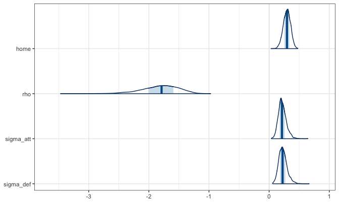
How to read the plot:
- each row is the estimated posterior density of a parameter, and the curve spans the whole range of the draws;
- the vertical line is the posterior median and the shaded area the central 50% credible interval (the defaults of
mcmc_areas(); use theprob,prob_outerandpoint_estarguments to change them).
The posterior of home is concentrated on positive values. The posterior of rho is the widest, extending from about \(-3.5\) to \(-1.0\), and skewed to the left (its mean, \(-1.82\), is lower than its median, \(-1.79\)). The posteriors of sigma_att and sigma_def are similar, bounded below by zero and slightly skewed to the right.
Other static models
The other models are selected through the model argument. The Dixon-Coles model adds the low-score dependence parameter \(\rho\), whereas the negative binomial model adds the dispersion parameters \(\phi_1\) (home) and \(\phi_2\) (away):
fit_dc <- stan_foot(
  data = italy_2000,
  model = "dixon_coles",
  chains = n_chains,
  parallel_chains = n_chains,
  iter_sampling = n_iter,
  seed = seed
)

fit_nb <- stan_foot(
  data = italy_2000,
  model = "neg_bin",
  chains = n_chains,
  parallel_chains = n_chains,
  iter_sampling = n_iter,
  seed = seed
)print(fit_dc, pars = c("home", "rho"))
#> Summary of Stan football model
#> ------------------------------
#>
#> Posterior summaries for model parameters:
#> # A tibble: 2 × 10
#> variable mean median sd mad q5 q95 rhat ess_bulk ess_tail
#> <chr> <dbl> <dbl> <dbl> <dbl> <dbl> <dbl> <dbl> <dbl> <dbl>
#> 1 home 0.41 0.411 0.046 0.046 0.333 0.485 1 4466. 2808.
#> 2 rho -0.071 -0.073 0.06 0.061 -0.167 0.031 1.00 4117. 1689.
print(fit_nb, pars = c("home", "phi1", "phi2"))
#> Summary of Stan football model
#> ------------------------------
#>
#> Posterior summaries for model parameters:
#> # A tibble: 3 × 10
#> variable mean median sd mad q5 q95 rhat ess_bulk ess_tail
#> <chr> <dbl> <dbl> <dbl> <dbl> <dbl> <dbl> <dbl> <dbl> <dbl>
#> 1 home 0.417 0.416 0.051 0.049 0.333 0.501 1.00 7278. 2766.
#> 2 phi1 12.0 11.7 2.82 2.82 7.77 17.0 1 7564. 3071.
#> 3 phi2 8.59 8.22 2.76 2.69 4.67 13.7 1.00 8350. 3115.- Dixon-Coles \(\rho\): the posterior mean is slightly negative (\(-0.071\)) and the 90% interval \([-0.167, 0.031]\) covers zero. The posterior is closer to zero than the MLE (\(-0.1627\)): in the Stan model \(\rho\) has a \(\mathrm{N}(0, 0.1)\) prior and is restricted to the interval \([-0.2, 0.2]\).
- Negative binomial dispersions: unlike the MLEs, the posterior means of \(\phi_1\) (12.0) and \(\phi_2\) (8.59) are finite. The likelihood is maximized as \(\phi \to \infty\), but in the Stan model the dispersions have half-normal \(\mathrm{N}^+(0, 5)\) priors, which put little mass on very large values. These values imply only a mild overdispersion: for instance, with a mean of 1.5 goals and \(\phi = 12\), the variance is \(1.5 + 1.5^2/12 \approx 1.69\).
Both results point to the double Poisson model as an adequate description of this season, at least with respect to these two extensions. This agrees with the maximum likelihood fits, where neither Dixon-Coles nor the negative binomial improved on the double Poisson.
The home effects of these two models (0.41 and 0.417, i.e. home scoring rates about 1.5 times the away ones for teams with the same abilities) are not directly comparable with the bivariate Poisson one (0.295), since in the latter the expected goals also include the covariance term: \(\text{E}(X) = \lambda_1 + \lambda_3\) and \(\text{E}(Y) = \lambda_2 + \lambda_3\). At the posterior means of fit_bp, two average teams have expected goals \(1.34 + 0.16 \approx 1.50\) at home and \(1 + 0.16 \approx 1.16\) away.
Changing the default priors
A common practice in Bayesian statistics is to change the priors and perform sensitivity tests. The prior_par argument of stan_foot() accepts a list with up to three elements; the elements that are not provided keep their default value:
| Element | Prior for | Default | Allowed families |
|---|---|---|---|
ability |
team-specific abilities (family and location) | normal(0, NULL) |
normal, student_t, cauchy, laplace |
ability_sd |
group-level standard deviations \(\sigma_{\text{att}}, \sigma_{\text{def}}\) | cauchy(0, 5) |
normal, student_t, cauchy, laplace |
home |
home effect | normal(0, 5) |
normal only |
The prior functions are documented in priors: normal(location, scale), student_t(df, location, scale), cauchy(location, scale) (equivalent to student_t with df = 1) and laplace(location, scale). Since the standard deviations are positive, the prior given in ability_sd acts as a half-distribution (e.g. the default is a half-Cauchy).
For instance, we may consider Student-\(t\) distributed abilities with 4 degrees of freedom and a half-Laplace prior for the standard deviations:
\[\begin{align} \text{att}_t & \sim t(4, \mu_{\text{att}}, \sigma_{\text{att}}), \qquad \text{def}_t \sim t(4, \mu_{\text{def}}, \sigma_{\text{def}}), \\ \sigma_{\text{att}}, \sigma_{\text{def}} & \sim \mathsf{Laplace}^+(0, 1). \end{align}\]
The scale of the abilities’ prior is not a fixed number but the group-level parameter \(\sigma_{\text{att}}\) (or \(\sigma_{\text{def}}\)), which is estimated with its own prior given in ability_sd. For this reason, the scale of the ability prior must be left as NULL: a numerical value is ignored, with a warning. The call below also widens the prior of the home effect to \(\mathrm{N}(0, 10)\):
fit_bp_t <- stan_foot(
  data = italy_2000,
  model = "biv_pois",
  prior_par = list(
    ability = student_t(4, 0, NULL),
    ability_sd = laplace(0, 1),
    home = normal(0, 10)
  ),
  chains = n_chains,
  parallel_chains = n_chains,
  iter_sampling = n_iter,
  seed = seed
)
We compare the marginal posteriors of \(\sigma_{\text{att}}\) under the default priors and under the alternative ones, binding the two columns of draws into a single matrix:
posterior_bp_t <- fit_bp_t$fit$draws(format = "matrix")
sigma_att_post <- cbind(
  posterior_bp[, "sigma_att"],
  posterior_bp_t[, "sigma_att"]
)
colnames(sigma_att_post) <- c("Default", "Student-t + Laplace")

color_scheme_set("gray")
mcmc_areas(sigma_att_post) +
  ggtitle("Posterior of sigma_att under two prior specifications") +
  theme_bw()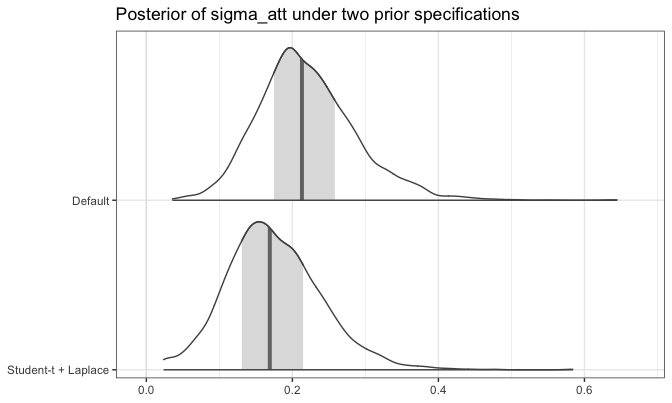
As before, the vertical lines are the posterior medians and the shaded areas the 50% credible intervals. Under the Student-\(t\) + Laplace specification the posterior of \(\sigma_{\text{att}}\) is shifted towards smaller values: the median moves from 0.213 to roughly 0.17.
This shift should be read with care, since the meaning of \(\sigma_{\text{att}}\) changes with the family of the abilities’ prior. Under the Gaussian prior it is the standard deviation of the attack abilities, whereas under the Student-\(t\) prior with \(\nu = 4\) degrees of freedom it is a scale parameter, and the standard deviation is \(\sigma_{\text{att}} \sqrt{\nu / (\nu - 2)} = \sqrt{2} \, \sigma_{\text{att}}\). At the medians, the implied standard deviation of the attack abilities is about \(\sqrt{2} \times 0.17 \approx 0.24\), similar to the 0.213 of the default specification. Comparing the scale parameters alone therefore does not show a larger shrinkage of the abilities. To assess the sensitivity of the conclusions, compare quantities with the same meaning under the two priors, such as the team abilities themselves (e.g. print(fit_bp_t, pars = "att")) or the predictions.
A few other ways of setting the priors:
# change only the prior of the group-level standard deviations:
# the abilities and the home effect keep their default priors
stan_foot(data = italy_2000, model = "biv_pois",
  prior_par = list(ability_sd = normal(0, 1)), seed = seed)

# Laplace (double exponential) abilities
stan_foot(data = italy_2000, model = "biv_pois",
  prior_par = list(ability = laplace(0, NULL)), seed = seed)
Alternative algorithms
The method argument selects the inference algorithm, among the four values described in Goal-based models in a nutshell:
method |
Algorithm | cmdstanr method |
Some of the arguments accepted through ... |
|---|---|---|---|
"MCMC" (default) |
Hamiltonian Monte Carlo | $sample() |
chains, parallel_chains, iter_warmup, iter_sampling, thin, adapt_delta, max_treedepth |
"VI" |
Automatic differentiation variational inference (Kucukelbir et al. 2017) | $variational() |
algorithm, iter, draws, output_samples |
"pathfinder" |
Pathfinder (Zhang et al. 2022) | $pathfinder() |
num_paths, draws, single_path_draws, max_lbfgs_iters |
"laplace" |
Laplace approximation | $laplace() |
mode, jacobian, draws, opt_args |
stan_foot() passes to cmdstanr only the arguments that are relevant to the selected method (plus seed), and silently drops the others: for instance, chains and iter_sampling have no effect with method = "pathfinder". The approximate algorithms are typically faster than HMC and can be useful for exploratory purposes. The following call uses the Pathfinder algorithm:
fit_bp_pf <- stan_foot(
  data = italy_2000,
  model = "biv_pois",
  method = "pathfinder",
  seed = seed
)print(fit_bp_pf, pars = c("home", "rho", "sigma_att", "sigma_def"))
#> Summary of Stan football model
#> ------------------------------
#>
#> Posterior summaries for model parameters:
#> # A tibble: 4 × 7
#> variable mean median sd mad q5 q95
#> <chr> <dbl> <dbl> <dbl> <dbl> <dbl> <dbl>
#> 1 home 0.278 0.269 0.048 0.039 0.214 0.354
#> 2 rho -1.71 -1.65 0.181 0.135 -2.01 -1.55
#> 3 sigma_att 0.201 0.186 0.034 0.018 0.165 0.264
#> 4 sigma_def 0.231 0.226 0.081 0.126 0.141 0.353The output has the same structure as before, but without the rhat, ess_bulk and ess_tail columns: these diagnostics refer to Markov chains, and the draws of the approximate algorithms ("VI", "pathfinder" and "laplace") are draws from an approximation of the posterior, not from Markov chains. As a consequence, the summaries do not tell how good the approximation is.
The comparison with the MCMC fit fit_bp is informative. The posterior means are similar to the MCMC ones (e.g. 0.278 against 0.295 for home, 0.231 against 0.23 for sigma_def), with sigma_att somewhat lower (0.201 against 0.22). However, the posterior standard deviations of home, rho and sigma_att are about 50-80% of the MCMC ones (e.g. 0.034 against 0.067 for sigma_att), and their 90% intervals are narrower accordingly (\([0.165, 0.264]\) against \([0.122, 0.341]\) for sigma_att). For sigma_def, in contrast, the standard deviation is slightly larger (0.081 against 0.071) and the 90% interval is close to the MCMC one (\([0.141, 0.353]\) against \([0.128, 0.357]\)). Here the approximation underestimates the posterior uncertainty of most parameters: approximate fits are useful for a quick exploration, whereas MCMC should be used for the final analysis, model checking and model comparison.
The other two approximate algorithms are called in the same way:
fit_bp_vi <- stan_foot(data = italy_2000, model = "biv_pois",
  method = "VI", seed = seed)
fit_bp_la <- stan_foot(data = italy_2000, model = "biv_pois",
  method = "laplace", seed = seed)
Practical notes
- Other arguments of
stan_foot().home_effect = FALSEremoves the home effect from the model;predictleaves the last matches out-of-sample (see Predictions);dynamic_typemakes the abilities time-varying (see Dynamic models);rankingadds a ranking covariate (see Bradley-Terry-Davidson). The full list is in the reference pages of stan_foot, mle_foot and print.stanFoot. - Data. Both functions require a data frame with the columns
periods,home_team,away_team,home_goals,away_goals; with more than five columns they issue a warning.mle_foot()fits static models only. - Priors. The prior of the home effect must be
normal(), otherwisestan_foot()stops with an error; any element ofprior_parother thanability,ability_sdandhomealso produces an error; a numerical scale in theabilityprior is ignored with a warning. print. A name inparsthat matches no parameter produces a warning, and a team name inteamsthat is not in the data is dropped with a warning; usedigits(default 3) to change the rounding.- Diagnostics. For MCMC fits,
fit_bp$fit$diagnostic_summary()reports the number of divergent transitions and of iterations that hit the maximum tree depth, which complement \(\hat{R}\) and the effective sample sizes. Graphical checks of the fitted models are shown in Model checking.